02. Haris Corner Detection
Harris Corner Detection
ND313 C03 L03 A04 C32 Intro
Local Measures of Uniqueness
The idea of keypoint detection is to detect a unique structure in an image that can be precisely located in both coordinate directions. As discussed in the previous section, corners are ideally suited for this purpose. To illustrate this, the following figure shows an image patch which consists of line structures on a homogeneously colored background. A red arrow indicates that no unique position can be found in this direction. The green arrow expresses the opposite. As can be seen, the corner is the only local structure that can be assigned a unique coordinate in x and y.
.png)
In order to locate a corner, we consider how the content of the window would change when shifting it by a small amount. For case (a) in the figure above, there is no measurable change in any coordinate direction at the current location of the red window W whereas for (b), there will be significant change into the direction orthogonal to the edge and no change when moving into the direction of the edge. In case of (c), the window content will change in any coordinate direction.
The idea of locating corners by means of an algorithm is to find a way to detect areas with a significant change in the image structure based on a displacement of a local window W. Generally, a suitable measure for describing change mathematically is the sum of squared differences (SSD), which looks at the deviations of all pixels in a local neighborhood before and after performing a coordinate shift. The equation below illustrates the concept.
.png)
After shifting the Window W by an amount u in x-direction and v in y-direction the equation sums up the squared differences of all pixels within W at the old and at the new window position. In the following we will use some mathematical transformations to derive a measure for the change of the local environment around a pixel from the general definition of the SSD.
In the first step, based on the definition of E(u,v) above, we will at first make a Taylor series expansion of I(x+u, y+u) . For small values of u and v, the first-order approximation is sufficient, which leads to the following expression.
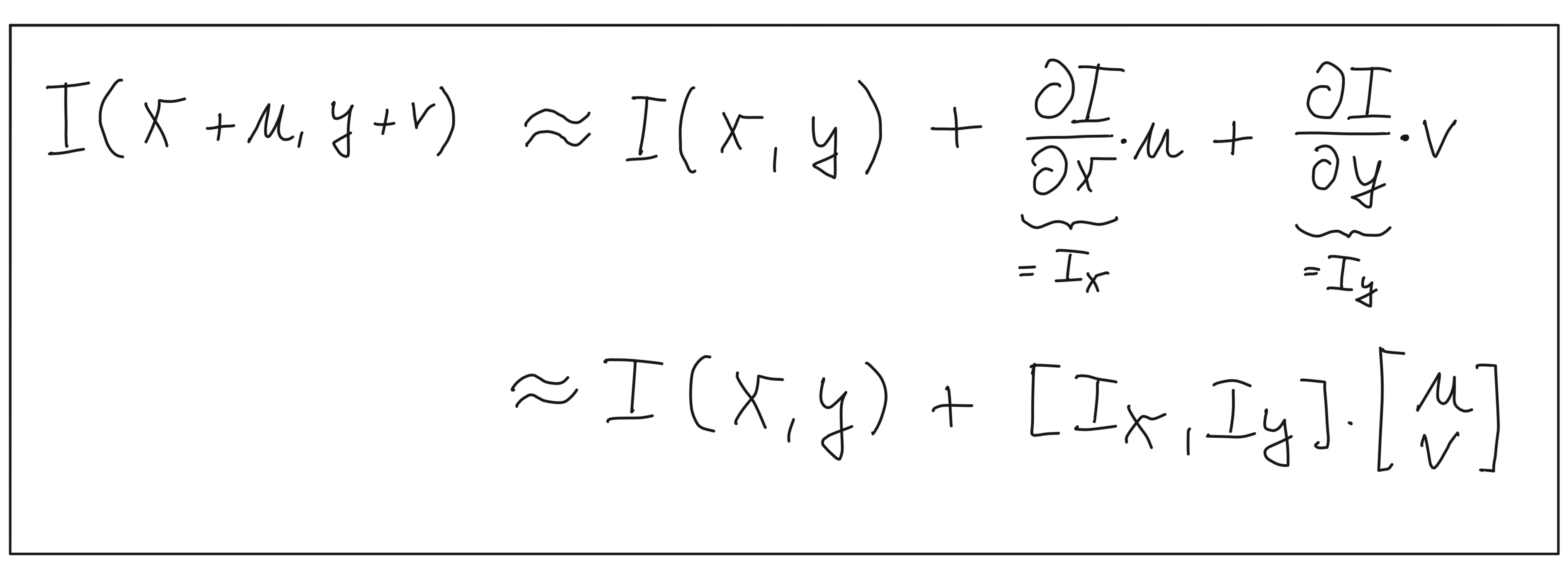
The derivation of the image intensity I both in x- and y-direction is something you have learned in the previous section already - this is simply the intensity gradient . From this point on, we will use the shorthand notation shown above to express the gradient.
In the second step, we will now insert the approximated expression of I(x+u, y+v) into the SSD equation above, which simplifies to the following form:
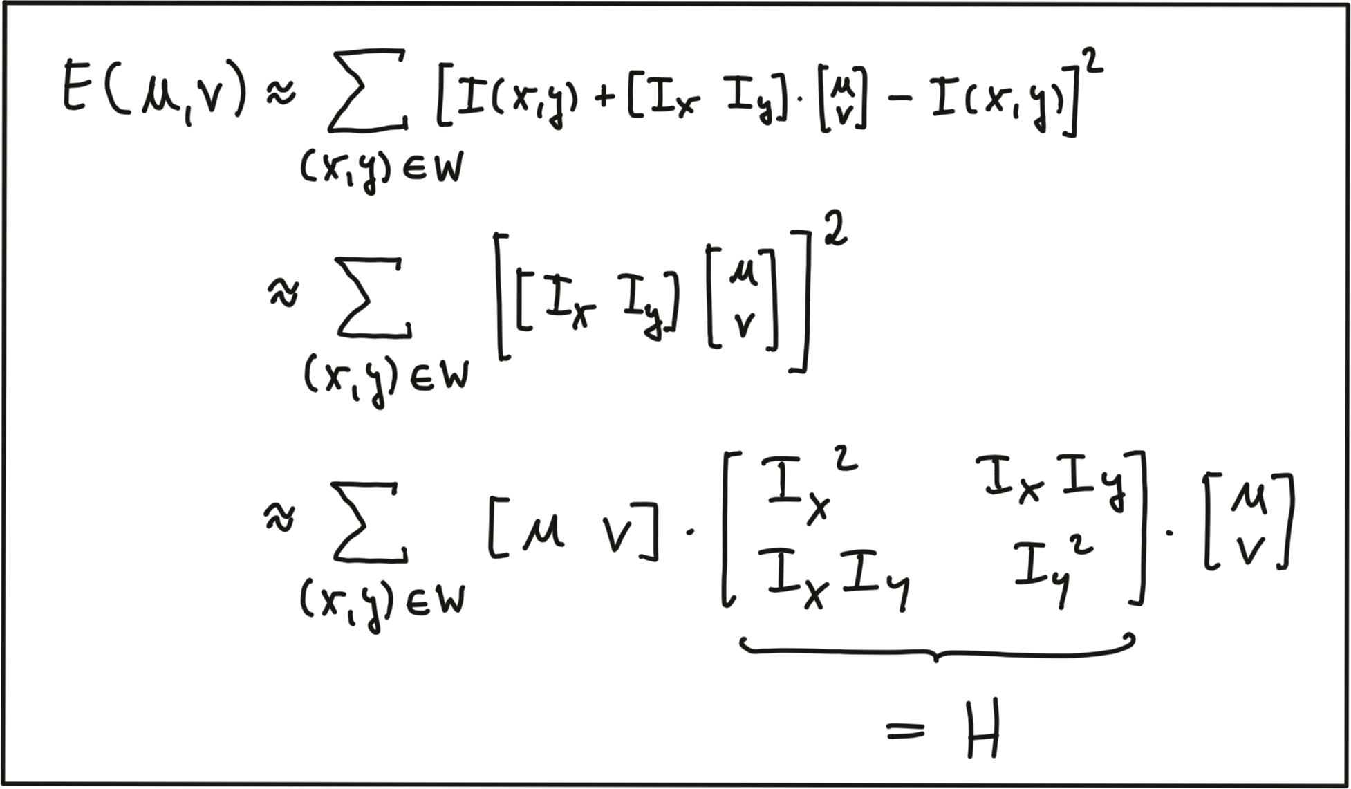
The result of our mathematical transformations is a matrix H , which can now be conveniently analyzed to locate structural change in a local window W around every pixel position u,v in an image. In the literature, the matrix H is often referred to as covariance matrix.
To do this, it helps to visualize the matrix H as an ellipse, whose axis length and directions are given by its eigenvalues and eigenvectors. As can be seen in the following figure, the larger eigenvector points into the direction of maximal intensity change, whereas the smaller eigenvector points into the direction of minimal change. So in order to identify corners, we need to find positions in the image which have two significantly large eigenvalues of H .
.png)
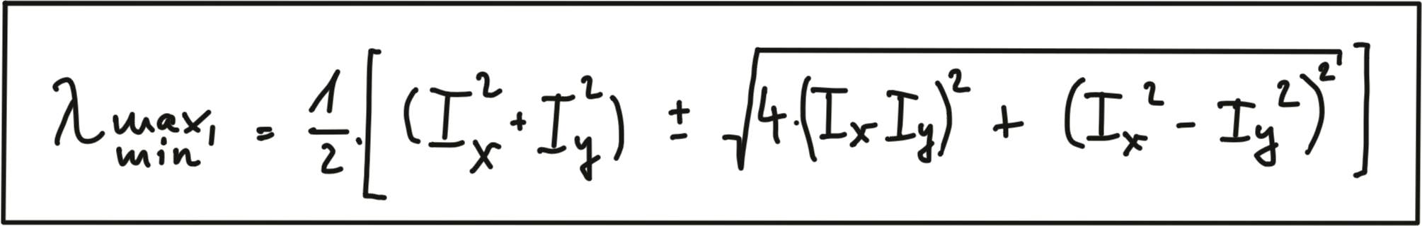
Without going into details on eigenvalues in this course, we will look at a simple formula of how they can be computed from H :
In addition to the smoothing of the image before gradient computation, the Harris detector uses a Gaussian window w(x,y) to compute a weighted sum of the intensity gradients around a local neighborhood. The size of this neighborhood is called scale in the context of feature detection and it is controlled by the standard deviation of the Gaussian distribution.
.png)
As can be seen, the larger the scale of the Gaussian window, the larger the feature below that contributes to the sum of gradients. By adjusting scale, we can thus control the keypoints we are able to detect.
The Harris Corner Detector
Based on the eigenvalues of H , one of the most famous corner detectors is the Harris detector. This method evaluates the following expression to derive a corner response measure at every pixel location with the factor k being an empirical constant which is usually in the range between k = 0.04 - 0.06.
.png)
Based on the concepts presented in this section, the following code computes the corner response for a given image and displays the result.
    // load image from file
    cv::Mat img;
    img = cv::imread("./img1.png");

    // convert image to grayscale
    cv::Mat imgGray;
    cv::cvtColor(img, imgGray, cv::COLOR_BGR2GRAY);

    // Detector parameters
    int blockSize = 2; // for every pixel, a blockSize × blockSize neighborhood is considered
    int apertureSize = 3; // aperture parameter for Sobel operator (must be odd)
    int minResponse = 100; // minimum value for a corner in the 8bit scaled response matrix
    double k = 0.04; // Harris parameter (see equation for details)

    // Detect Harris corners and normalize output
    cv::Mat dst, dst_norm, dst_norm_scaled;
    dst = cv::Mat::zeros(imgGray.size(), CV_32FC1 );
    cv::cornerHarris( imgGray, dst, blockSize, apertureSize, k, cv::BORDER_DEFAULT );
    cv::normalize( dst, dst_norm, 0, 255, cv::NORM_MINMAX, CV_32FC1, cv::Mat() );
    cv::convertScaleAbs( dst_norm, dst_norm_scaled );

    // visualize results
    string windowName = "Harris Corner Detector Response Matrix";
    cv::namedWindow( windowName, 4 );
    cv::imshow( windowName, dst_norm_scaled );
    cv::waitKey(0);
The result can be seen below : The brighter a pixel, the higher the Harris corner response.
.png)
Exercise
ND313 C03 L03 A05 C32 Outro
In order to locate corners, we now have to perform a non-maxima suppression to (a) ensure that we get the pixel with maximum cornerness in a local neighborhood and (b) to prevent corners from being too close to each other as we prefer an even spread of corners throughout the image.
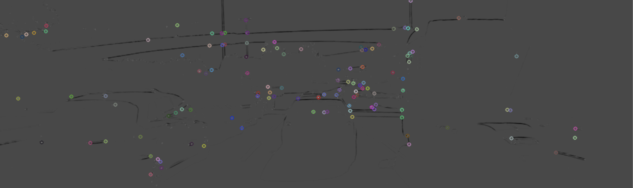
Your task is to locate local maxima in the Harris response matrix and perform a non-maximum suppression (NMS) in a local neighborhood around each maximum. The resulting coordinates shall be stored in a list of keypoints of the type
vector<cv::KeyPoint>
. The result should look like this, with each circle denoting the position of a Harris corner.
You can write your code in the
cornerness_harris.cpp
file in the desktop workspace below. After building, you can run the code using the generated
cornerness_harris
executable.
Workspace
This section contains either a workspace (it can be a Jupyter Notebook workspace or an online code editor work space, etc.) and it cannot be automatically downloaded to be generated here. Please access the classroom with your account and manually download the workspace to your local machine. Note that for some courses, Udacity upload the workspace files onto https://github.com/udacity , so you may be able to download them there.
Workspace Information:
- Default file path:
- Workspace type: react
- Opened files (when workspace is loaded): n/a
-
userCode:
             export CXX=g++-7


              export CXXFLAGS=-std=c++17